Introduction to GANS Part 1/2
This introduction is assuming you have a basic understanding of Neural Networks, activation functions, and the likes. To begin let us go over the general idea behind activation functions, batch normalization, padding, stride, pooling, upsampling and downsampling.
Activation Functions:
Activations are functions that takes in a real number as input (knows as the Domain) and outputs a number within the range of the function. These activation functions (should be) nonlinear differential equations. These functions are usually set for a given layer within a network it is usually computed as
$$z_i^L = \sum_{i=0}W_i^L a_i^{L-1} + b^L$$where i is the node, L is the layer, W is the weights, b is the bias of the current layer and a is the output of the pervious layer. Since $a$ is the output of the grevious later is can be written as
$$a_i^L = g^L(z_i^L)$$where g is the activation function we assigned. Thus putting it all together we get the output of a given layer is
$$z_i^L = \sum_{i=0}W_i^L g^{L-1}(z_i^{L-1}) + b^L$$Since the activation function g is differential, we can find the gradient and implement backpropigation; furthermore since it is non-linear we can find more complex features. Some common activation functions are:
ReLU: (Rectified Linear Unit) $$g^L(Z^L) = max(0,Z^L)$$
import matplotlib.pyplot as plt
import numpy as np
x = np.random.uniform(-2,2,10000)
y = [max(0,i) for i in x]
plt.title("RELU")
plt.axhline(0, color='black')
plt.axvline(0, color='black')

plt.scatter(x,y)
<matplotlib.collections.PathCollection at 0x7fcebc2e3790>
One problem that occurs is with the dying ReLU problem, this is because ReLU has a derivative equal to zero when the output is zero; this will force the weights to stop learning and never be optimized. Which in turn will propigate down the network to other layers.
Leaky ReLU: $$g^L(Z^L) = max(a z^L,Z^L) \text{ s.t } 0 < a < 1$$
x = np.random.uniform(-2,2,10000)
y = [max(.1*i,i) for i in x]
plt.title("Leaky RELU")
plt.axhline(0, color='black')
plt.axvline(0, color='black')

plt.scatter(x,y)
<matplotlib.collections.PathCollection at 0x7fce9bd88390>
This solves the dying ReLU problem by adding a small slope (a) where a is a hyperparameter
Sigmoid $$g^L(Z^L) = \frac{1}{1+e^{-z^L}}$$
x = np.random.uniform(-5,5,10000)
y = 1/(1 + np.exp(-x))
plt.title("Sigmoid")
plt.axhline(0, color='black')
plt.axvline(0, color='black')

plt.scatter(x,y)
<matplotlib.collections.PathCollection at 0x7fce9bdb0dd0>
where the range is between zero and one, and the inflection point is at .5; this kind of activation function isnt usually used in hidden layers, but rather the output layer. This is because the range can be used in binary classification where the output is the probablitity of success (1 for yes, 0 for no). Also as you approach out outer limit of the function the derivative gets super small. This is commonly know as the vanishing gradient problem where, similar to the dying ReLU problem it can stop the node from learning.
Batch Normalization:
It should be common knowledge that the more different the data, the easier it is to classify. However sometimes data can have a very close distribution. For example if you have two parameters $x_1, x_2$ and $x_1$ is normally distributed, but $x_2$ is has a tight distribution, then we can see a graph of something like such
fig = plt.figure(figsize=(6,5))
left, bottom, width, height = 0.1, 0.1, 0.8, 0.8
ax = fig.add_axes([left, bottom, width, height])

start, stop, n_values = -20, 20, 800

x_vals = np.linspace(start, stop, n_values)
y_vals = np.linspace(start, stop, n_values)
X, Y = np.meshgrid(x_vals, y_vals)


Z = np.sqrt(2*X**2 + 10*Y**2)

cp = plt.contourf(X, Y, Z)
plt.colorbar(cp)

ax.set_title('Contour Plot where x_2 is highly corralated')
ax.set_xlabel('x_1')
ax.set_ylabel('x_2')
plt.show()
where is might be more difficult to find an optimal value, but if the input $x_1, and x_2$ is normalized, then training might be more easier and much faster
fig = plt.figure(figsize=(6,5))
left, bottom, width, height = 0.1, 0.1, 0.8, 0.8
ax = fig.add_axes([left, bottom, width, height])

start, stop, n_values = -20, 20, 800

x_vals = np.linspace(start, stop, n_values)
y_vals = np.linspace(start, stop, n_values)
X, Y = np.meshgrid(x_vals, y_vals)


Z = np.sqrt(X**2 + Y**2)

cp = plt.contourf(X, Y, Z)
plt.colorbar(cp)

ax.set_title('Contour Plot with similar corallations')
ax.set_xlabel('x_1')
ax.set_ylabel('x_2')
plt.show()
Padding and stride:
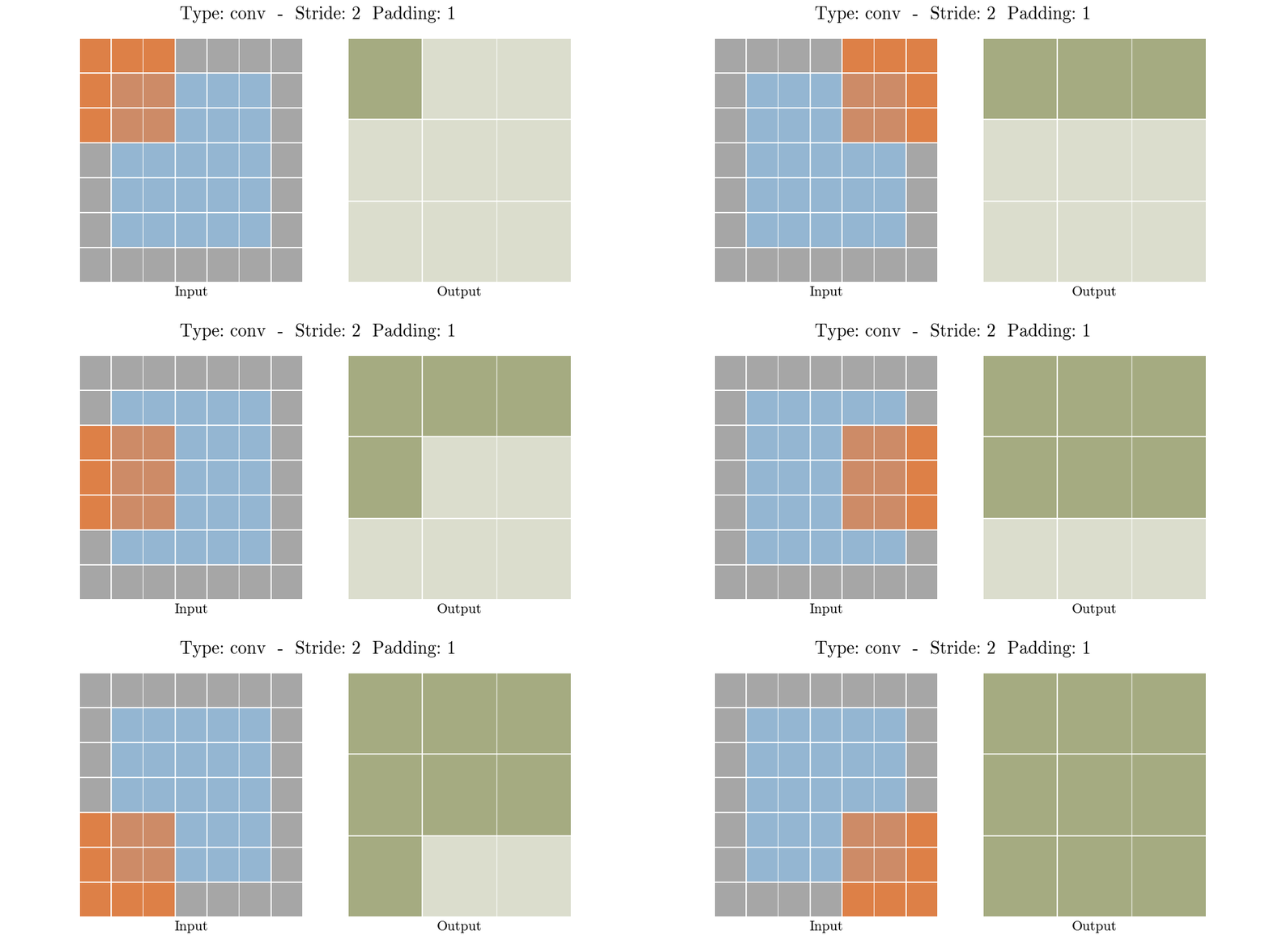
for a given NxM matrix, the stride would be how you move in order to do the convolution of a given area, while the padding is adding extra spaces on the edges of the matrix. A good look at learning more about these can be found here

Pooling
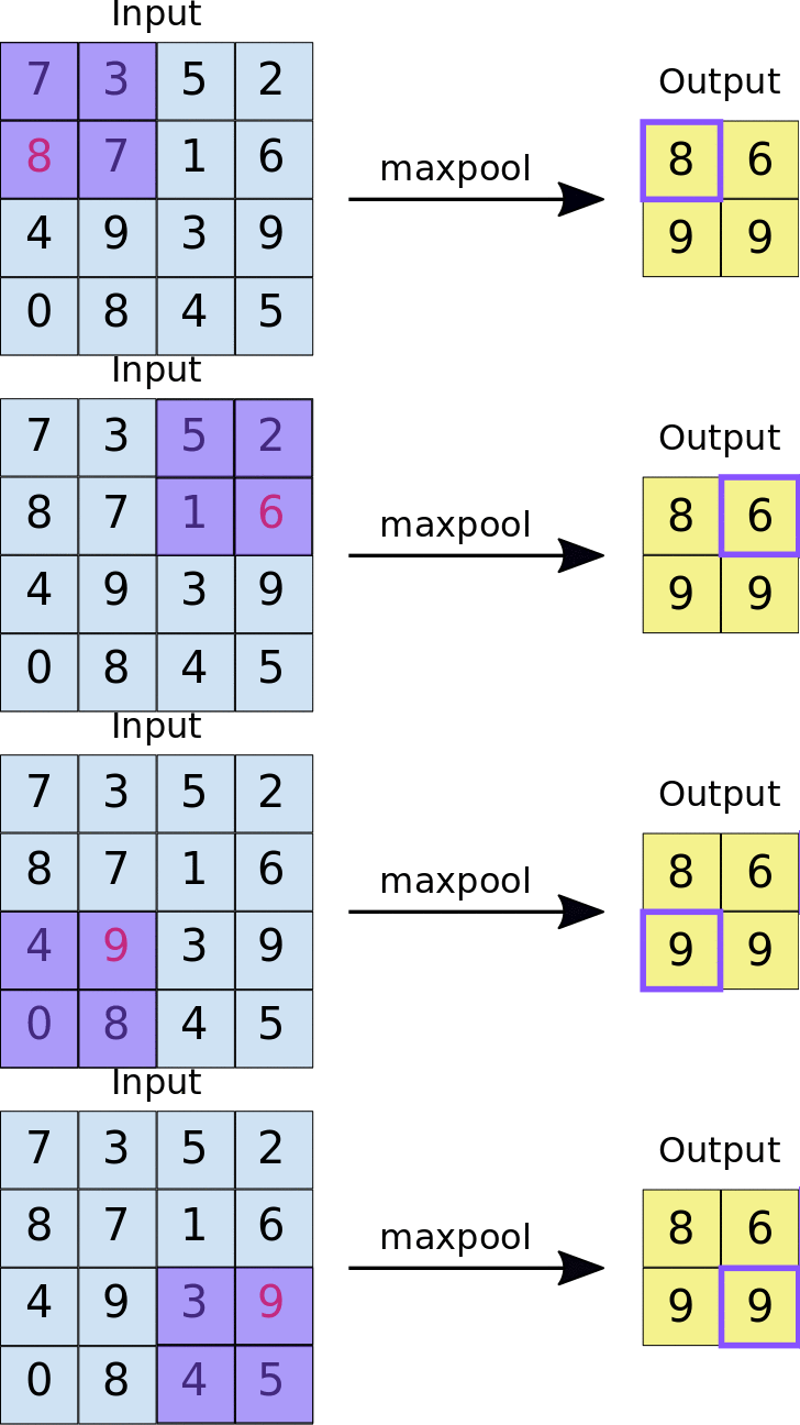
Pooling is used to reduce the size of the input and is commonly used in Neural Network. Pooling essentially reduces the size of a neural network this can be by taking a region of the input (in this case lets assume an image) and then applying some equation to reduce the size, one example would be max pooling, where we would only save the largest number in the "pool" (see below for an example)

Upsampling:
increasing the size of a image, but keeping the proportion of the pixels in the same format.

