The study of graphs have received a lot of attention over the years due to their ability to represent data. From Dijkstra’s algorithm to determine the shortest path between two points, plotting genomes, and even social networks graphs can play an important part in visualizing data. This is where the study of Graph Convolution Networks comes in. An example can be showed as such:
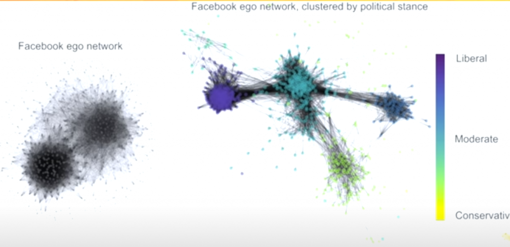
Figure 1: a Facebook Friendship network. Color indicates the political viewpoint of each friend; 10% of these political stances are predicted by graph convolutional network, the rest were input as part of the training sequence
An application of a Graph Convolution Network (GCN) can be shown as follows:
Given a Facebook users friends history (i.e links, shares, relationships, and such), we can create an unstructured graph of how they are related (as shown on the left-hand side, color: gray)
Using a GNC community clustering algorithm we can classify each person in the left-hand graph by their political stances.
Other examples can range from fraud detection, computer vision and so much more! These GCN’s are very powerful for learning on graphs. Formally, a graph convolution network(GCN) operates of a given graph G = (V,E) where V represents the Vectors and E represents the Edges.
Background: Graphs and Convolutions and Machine Learning!
Graphs:
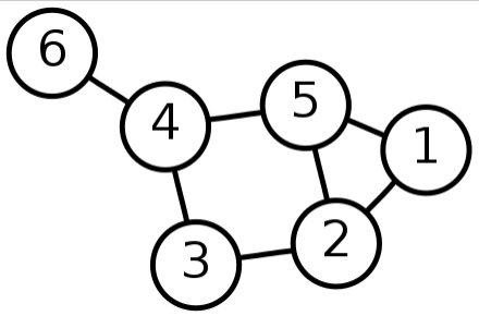
In mathematics, a graph is essentially a structure of objects that are interconnected. As seen in figure 2 almost every graph has vertices and edges at minimum.
There are a wide range of graphs Null , Connected, Bipartite, Weighted, and Directed to name a few. Each of these graphs can be extremely useful for visualizing data.
Figure 2: A simple graph with six vertices and seven edges
A down side to graphs are that comparing two graphs could be [katex] N^2[/katex] time because we need to check every Node and vertices. Not only that the graph can grow exponentially based on how many edges a new vertices takes on.
Convolutions
Figure 3: the convolution of the function f(x) interacting with a pulse, g(x)
Turning over to Convolutions, given two function F(x) and G(x) a convolution is a mathematical operation that produces a different function that shows how G(x) and F(x) interact with each other. Figure 3 represents a one dimensional convolution of a sliding function (red) interacting with a static function (blue). It is given by the function [katex]f(x) * g(x) = \int^{+\infty}_{-\infty} f(y) – g(x -y) \, dy[/katex]
Figure 4 shows the visualization of a two dimensional Convolution, which is commonly used in image processing and classification to reduce data size with minimal feature loss. We can combine the region of interest (dark blue) by using different kernel techniques.This in turn allows us to change the image without huge data loss
Figure 4: A convolution of a 4 x 4 image produces a 2 x 2 image
#Load imports
import numpy as np
import cv2
from matplotlib import pyplot as plt
from scipy import ndimage

# get grayscale image
image = cv2.imread("---image_location---", cv2.IMREAD_GRAYSCALE)

# show image
plt.imshow(image, cmap='gray', vmin=0, vmax=255)

# define kernel
kernel = (1/9) * np.array([[1, 1, 1],
                           [1, 1, 1],
                           [1, 1, 1]])

# apply kernel
filtered = cv2.filter2D(src=image, kernel=kernel, ddepth=-1)

# show new image
plt.imshow(filtered, cmap='gray', vmin=0, vmax=255)
Figure 5: A gray scale image of me
Figure 6: A gray scale image of me after applying a box blur kernel convolution
Machine Learning
Machine learning (ML) is the process of human developed models using data to auto tune its own parameters. George Box, a famous statistician once said “All models are wrong, some are useful” and this applies well to machine learning.
Some basics of ML in respect to the GCN are as follows
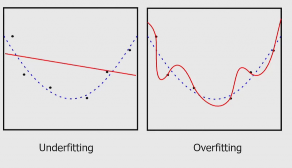
Supervised Machine Learning: given an input dataset [katex] \{ (x_1 , y_1) , … , (x_N , y_N) \}[/katex] find a function such that [katex] f(x_{theta}) = y_{theta}[/katex] or minimize the loss (within reason) between what is predicted and what the actual result is. An example of over or under fitting the loss can be shown in Figure 8
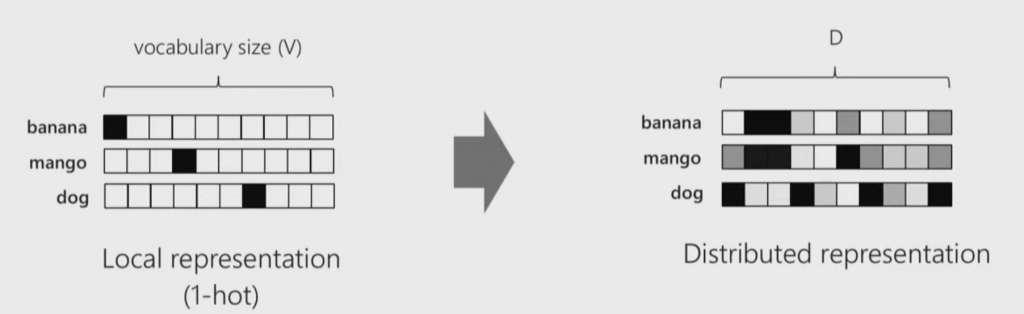
Distributed Vector Representations: given a set of discrete classifications we can one hot encode them such that it is easy to identify each input. Instead we take this forward and multiply a given one hot encoded matrix with a distribution matrix such that we can identify correlations between classifications (as seen in Figure 7).
Figure 7: transformation of a one hot encoding to a distributed representation
Figure 8: given the datapoints (blue dots) and the actual best fit (dotted line) we show the downside of not fitting or overfitting the loss function
Big Problem with Graphs:
Give any graph its dimension is at minimum n such that there exists a “classical representation” of the graph with all the edges having unit length. This means that said graph initially lies in N-Dimensional space and the size grows as you add more vertices.
Given an initial graph that represents a given problem where each node holds data we ask yourself the question:
The equation of a GCN is [katex inline=true] H^{l+1} = \sigma * \{ \hat{D}^{-\frac{1}{2}} \hat{A} \hat{D}^{-\frac{1}{2}} H^{(l)} W^{(l)} \} [/katex]
Where:
W is the Weights (trainable parameters),
A is the Adjacency matrix,
D is the Degree matrix (number of connections that attach to each node),
H is the current (Hidden) layer,
[katex inline=true] \sigma [/katex] is an activation function.
A GCN can be used for making classification decisions based on the the the nodes and edges on a graph. More information can be found here: Kipf, Thomas N., and Max Welling. “Semi-supervised classification with graph convolution networks.” arXiv preprint arXiv:1609.02907 (2016).